1. Stochastic vs Deterministic: Traditional software (referred to as software 1.0) operates deterministically, meaning it consistently produces the same output for a given system and input. In contrast, AI software (referred to as software 2.0) is stochastic, meaning it can yield varying outputs for the same system and input.

   As a product manager, meticulous control over the user experience is paramount, especially to prevent negative user experiences. In the realm of software 1.0, this entails thorough scenario planning within the Product Requirements Document (PRD) to anticipate and design for potential errors. Once the software undergoes comprehensive testing, scenarios that pass ensure a reliable user experience in production, barring any unforeseen bugs.

   However, the landscape shifts with AI software (software 2.0). Even after rigorous testing, AI systems may still generate incorrect responses due to their stochastic nature. Such occurrences are not considered bugs but rather inherent to the probabilistic framework of AI software. Acknowledging that no AI system achieves perfect accuracy, product managers must proactively devise user experiences capable of managing errors and gracefully handling failures. This necessitates a specialized understanding of AI design processes for product managers to effectively navigate this terrain.

2. Designing for loops (control loop, feedback loop, human-in-the-loop): Given the stochastic nature of AI systems, errors are inevitable. As a product manager, it's imperative to establish control loops to swiftly determine whether the AI's output is beneficial to the end user. If not, end users should be empowered to take control of the system to override the AI's decisions, stop AI recommendations.

   Similarly, the product team must institute feedback loops for each AI feature to assess its efficacy for end users. This involves gathering data across various scenarios to ascertain when the feature performs optimally and when it falters.

   Additionally, designing for humans-in-the-loop is crucial, enabling the seamless transition of control from AI systems to human operators when necessary.

3. Data Collection: It's widely recognized that AI relies heavily on data. However, the responsibility of data collection doesn't fall on AI scientists; rather, it lies with the product team. Why? Because the product team holds ownership of the product, making them best suited to embed the necessary instrumentation for data collection.

   This is where PMs need to understand the lingo of data systems and work with data engineering teams to create roadmaps & sprints for data collection. In large AI first MNCs, this is a very specialized role called Data PM.

4. Introducing Users to AI: When integrating AI into your products for the first time, it's vital to introduce AI to your users delicately. Setting the right expectations and assuring users that they can regain control if they're uncomfortable is essential. Achieving this demands the creation of a highly specialized flows & UX.

5. Economics of AI: AI constitutes a costly endeavor, encompassing expenses in data acquisition, cleaning, storage to create datasets; computational resources, and talent acquisition. Given the high costs involved, not every potential use case justifies the investment. Hence, it's imperative to select use cases judiciously.

   Within a company, the business team comprehends business dynamics but often lacks technical expertise, while individual contributors (ICs) in the AI team possess technical proficiency but may not grasp business intricacies. In this landscape, product managers play a pivotal role, bridging the gap between technology, user needs, and business objectives. Consequently, the responsibility of evaluating and determining the feasibility & viability of AI use cases predominantly falls on the shoulders of product managers.

6. The AI development process is very different: The transition from traditional software development (Software 1.0) to AI-driven systems (Software 2.0) introduces significant differences in how product management approaches roadmaps and timelines. Here are some implications for product owners:
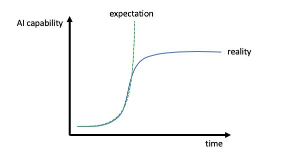
   • Uncertainty in Improvement: Unlike traditional software where incremental improvements are often achievable by addressing specific issues or corner cases, AI-driven systems may hit performance plateaus where further improvements are challenging. This uncertainty must be factored into product roadmaps and timelines, as achieving desired performance levels may require more extensive reevaluation and experimentation.
   • Extended Development Cycles: Improving AI-driven systems often involves revisiting the underlying algorithms, data pipelines, or model architectures, which can be time-consuming processes. Product owners need to allocate sufficient time in their roadmaps for research, experimentation, and validation of new approaches, potentially extending development cycles beyond what is typical for traditional software updates.
   • Resource Allocation: Given the longer development cycles associated with improving AI systems, product owners may need to allocate additional resources, both in terms of engineering talent and computational resources. This may require reprioritizing other initiatives or increasing investment in AI research and development to meet performance targets within the desired timeframe.

Key Lessons:

• You can have the most cutting-edge technology which even your competition tries to copy, yet if it doesn’t move business needles it is a liability.
• Business & Product took a leap of faith that users will order goods purely using voice without even looking at items even once. This and other monetization efforts didn’t happen and everything fell apart.
• Mistakes made by the product team are super expensive. PMs must find ways to list down and validate assumptions, especially leap of faith, as quickly as possible. In the case of Alexa, I wonder if there were ways to test these without having to invest so much time & effort.
• Alexa single-handedly contributed to so many developments in speech tech, it is an absolute marvel. Yet reduced only to alarms, how is the weather outside and play song. Primarily due to points (2) and (3).
• Business needs to understand that building cutting-edge tech takes time - no matter how much you may push, it can't be done in days, weeks or sometimes even months.

• Organizations must clearly specify minimum working hours they expect. Be explit, say Mon-Fri (10am-7pm) or watever works for them. Be reasonable - dont say 24 hrs a day, 7 days a week!
• In their free time, employees should be free to pursue their interests - some like to chill n watch Netflix, others like to work on side gigs. That should be entirely employee’s choice - no organizations should not dictate this
• Organizations should make moonlighting policy super transparent. Create a system where employees must inform of all side gigs to the employer. In return, employers must not object to side gigs unless there is a clear conflict of interest.
• Organizations should evaluate employees purely on their performance in their organization. If the performance is great, reward them accordingly. If not, put them on PIP or let them go. Unless a side gig is clearly impacting an employee’s performance - it should not concern the employer.
• Employees must understand companies will be more transparent only if employees don’t cheat. So:
  • Only 1 full-time employment. Can’t take 2 overlapping jobs. To be more precise - time commitment of one job must not conflict with time commitment of any other gig.
  • Employee can have side gigs but only in your free time (time not commited to organization).
  • Employee must inform of all side gigs to employer.
  • Employers must not object to side gigs unless there is a clear conflict of interest.
  • Employees’s side gig cannot be with competitor companies for up to 1 yrs (maybe even 2 years) after leaving any employer. Organizations must have a strong right to protect IP, business strategy, internal details etc. Any clear conflict of interest must be strictly prohibited.
• Despite all this, if an employee moonlighting, Organizations should have the legal right to take a very strict action and penalize them heavily.

• Finding the right use case: finding a problem that is important to its users and can be solved well by AI. I talked earlier on this here

• Having the right data: most companies have tonnes of data but seldom have the data for the problem at hand. In AI its not just the quantity of data that matters but also the quality of data. Do you have the training data that resembles the production data very closely? Does it have enough data points that represent various outliers, mean data points, data points near the actual decision boundary etc
• Labeling cost - If you need to get your data manually labeled, this will need lots of time and money. The process of labeling itself might not be straightforward. How do you benchmark the quality of labeling? If your labelers are making mistakes this can jeopardize the entire project.
• Compute cost - the cost of the compute needed for training the model and for inference. This is especially crucial if your solution uses deep learning.
• Going from a solution to the solution: In AI there is no one way to solve a problem. There are multiple ways and each will give you a different accuracy. Getting from the point where you have a model that gives you an acceptable performance to getting to a model that gives you fabulous performance is often a very long journey.
• Fitting model into the product to get AI-driven feature: Its not just a simple API integration. One needs to figure out the best UX to serve the predictions, should this UX be intrusive or soft suggestions, UX should be able to gracefully handle the scenarios when the model makes mistakes, a mechanism to let the human take over when it is going all wrong for the end-user, instrumentation to collect data to continuously evaluate the performance of the model on prod data, instrumentation to collect data for future modeling efforts.
• Need to retrain model: many times AI systems require one to retrain the model after every 15-30 days on the latest data.
• Talent: DS/ML team alone cannot pull off all the above. You need good and diverse talent for this - ML/DS folks who can evaluate the various approaches depending on the situation and can take the most suitable one to build the right model (and not blindly apply DL), Data engineers to build data pipelines to collect all data, a product manager who can figure out right use case, build instrumentation, UX to handle mistakes, a AI leader who understands this entire life cycle and work very closely with business and speak their language. This talent doesn’t come cheap.

• Finding newer uses cases and touch points in your product(s) where AI can deliver a completely new experience to the user : This innovation often create USP/key differentiator for the product compared to the competition in the respective segment. And if the feature is killer, it changes the user’s behavior which in turn changes user expectation. And then the competition has no other option but to play the catch-up game. This creates a very strong moat. For example, YouTube uses AI to generate subtitles in multiple languages on the fly. They have fundamentally changed user expectations and other platforms have to have a similar feature.

  This kind of innovation is often not as easy as it may sound. I have written about this in an earlier post (ref : Hobbiton - Uses cases where AI can deliver great returns). This requires first principle thinking. Product managers who can envision features in a completely new way using AI, very close collaboration between AI & product teams to understand what is possible what is not, a very good execution to deliver A-class experience (despite AI model will make mistakes).

• Building the dataset for the problem at hand : For AI teams embedded in product settings, building a comprehensive dataset for the problem at hand is often 80% of the battle. Building such a dataset is never writing a bunch of queries on a massive data store at your disposal. AI Teams often have to come up with very smart strategies, hacks to augment data to arrive at a comprehensive dataset. Also, this is not a one-time activity but often highly iterative. What more type of data is needed - comes from the kind of mistakes your models are making.

  I will soon be writing a dedicated post on some of the best examples I have seen/heard on innovative ideas to collect data.

• Publishing paper/patent (doesn’t happen that often) : AI teams embedded in product teams do write patents and papers - but this is seldom their true north star.

• Articles on AI in popular media with lofty claims (remember the humanoid dancing in Tesla AI day or Sophia - not many people understand these are mere marketing and perception gimmicks)
• The thought that AI at the end of the day is a code - so it cannot be very different from software engineering. The issues are mere initial hiccups which is always the case with any new tech, so is the case with AI

So most leaders expect the ROI curve in AI to be a vertical takeoff. This expectation is further fueled by the fact that AI doesn’t come cheap - data, data engg & AI teams, talent cost, hardware cost, data collection & labeling cost and time etc, MLOps etc Read my previous write up titled the economics of AI

This is where most Orgs/Teams make THE mistake. The true ROI curve in AI is very very different from their expectations. As shown in the figure below, it follows a S shape curve.

• Initial lower part of S: One needs to invest a lot of time and energy with very little ROI - finding the right use case, right quality and quantity of data and labels (more on this in another post), right modeling approach, right metrics etc. This can take anywhere between 1-3 years.
• Middle part of S: This is where one gets the highest ROI per unit effort. This is because most of the hard work has been done in the first 1-3 years. All key stakeholders have a better understanding of the AI journey. This phase is all about building the 2nd/3rd version of AI systems
• Later upper part of S: This is where the ROI again starts to stagnate. This phase is where your team is building the 6th/7th version of the system and trying to push systems performance to the upper 90s. This often requires completely new approaches, new algorithms. Its not just adding a couple of lines of code!

• Finding the right use case: finding a problem that is important to its users and can be solved well by AI. I talked earlier on this here

• Having the right data: most companies have tonnes of data but seldom have the data for the problem at hand. In AI its not just the quantity of data that matters but also the quality of data. Do you have the training data that resembles the production data very closely? Does it have enough data points that represent various outliers, mean data points, data points near the actual decision boundary etc
• Labeling cost - If you need to get your data manually labeled, this will need lots of time and money. The process of labeling itself might not be straightforward. How do you benchmark the quality of labeling? If your labelers are making mistakes this can jeopardize the entire project.
• Compute cost - the cost of the compute needed for training the model and for inference. This is especially crucial if your solution uses deep learning.
• Going from a solution to the solution: In AI there is no one way to solve a problem. There are multiple ways and each will give you a different accuracy. Getting from the point where you have a model that gives you an acceptable performance to getting to a model that gives you fabulous performance is often a very long journey.
• Fitting model into the product to get AI-driven feature: Its not just a simple API integration. One needs to figure out the best UX to serve the predictions, should this UX be intrusive or soft suggestions, UX should be able to gracefully handle the scenarios when the model makes mistakes, a mechanism to let the human take over when it is going all wrong for the end-user, instrumentation to collect data to continuously evaluate the performance of the model on prod data, instrumentation to collect data for future modeling efforts.
• Need to retrain model: many times AI systems require one to retrain the model after every 15-30 days on the latest data.
• Talent: DS/ML team alone cannot pull off all the above. You need good and diverse talent for this - ML/DS folks who can evaluate the various approaches depending on the situation and can take the most suitable one to build the right model (and not blindly apply DL), Data engineers to build data pipelines to collect all data, a product manager who can figure out right use case, build instrumentation, UX to handle mistakes, a AI leader who understands this entire life cycle and work very closely with business and speak their language. This talent doesn’t come cheap.

Google used a very simple but powerful observation - most users can very easily recall how the special character that they need looks like, unlike their name. So, they provided a small sketch pad for users to draw what they remember and use the concepts from computer vision (Sketch-RNN) to suggest a few closest options based on the visual match. The same concept was later used to power Auto draw.

I often use this example to drive home the point that one often needs to think from first principles when thinking of AI-powered use cases. For the above-mentioned example, the more you think the more you will realize:

• The problem could not have been solved by traditional engineering approaches.
• It is a very well-defined narrow problem statement.
• The core AI concept (Sketch-RNN) was just right to solve this problem statement well.
• The solution (powered by AI in this case) really helped to solve the user’s pain point and deliver happiness.

This is especially useful in machine learning, where you want to visualize how a particular property of model/data evolves with time (training) Our matrix is of MxN dimensions, initialised randonly.

gunicorn server up and running Lets hit the server with a POST request. Open another terminal window and type in:

All the code in the snippets above can be found in the following jupyter notebook. If you face any issue with the code, please open a New issue on Github.

• In this post we will focus on the maths that goes into computing these gradients - we will systematically derive gradients. The complexity of calculations depends on 3 things:

  • Depth of the network
  • Number of training examples (1 or more)
  • Number of components in input (1=scalar, >1=vector)

  Through out this post we assume:

  • There is no bias term.
  • `.` is matrix multiplication, `*` is element wise product and `X` is normal multiplication.
  • All activations are sigmoid a.k.a logistic. It is defined as \( f(u) = \frac{1}{1+e^{-u}} \). If you plot it, it comes as:.

  

Sigmoid function

It easy to see it is smooth and differentiable and bound between 0 and 1 [No? not straight forward - need to fix this].

\[ \begin{align} \frac{d}{dx}\sigma(x) &= \frac{d}{dx} \left[ \frac{1}{1+e^{-x}}\right] \label{refB} \tag{B}\\ &= \frac{d}{dx} (1+e^{-x})^{-1} \\ &= -(1+e^{-x})^{-2}(-e^{-x}) \\ &= \frac{e^{-x}}{(1+e^{-x})^2} \\ &= \frac{1}{(1+e^{-x})} \cdot \frac{e^{-x}}{(1+e^{-x})} \\ &= \frac{1}{(1+e^{-x})} \cdot \frac{1 + e^{-x} -1}{(1+e^{-x})} \\ &= \frac{1}{(1+e^{-x})} \cdot \left( 1 - \frac{e^{-x}}{(1+e^{-x})} \right) \\ &= \sigma(x)(1-\sigma(x)) \label{refC} \tag{C} \end{align} \] \[ \begin{align} \frac{d}{dx}\sigma(ax) = a(\sigma(ax))(1-\sigma(ax)) \label{refD} \tag{D} \end{align} \]

We will be using the above result a lot, so make sure you understand it. If it is not clear, have a look at this post .

To compute the gradients, we will start with the simplest case and increase the complexity gradually. To keep things simple we will complete it in 7 parts
• 1 layer network, 1 training example (scalar).
• 1 layer network, 1 training example (vector)
• 1 layer network, batch training (>1 training examples where each is a vector)
• 2 layer network with 1 node hidden layer, 1 training example (vector
• 2 layer network with 2 node hidden layer, 1 training example (vector)
• 2 layer network, batch training (>1 training examples where each is a vector)
• Generalization and take home

Since we will be dealing with matrices, a key step in every equation is to check if all matrix dimensions are consistent.